A Student's Guide to Software Engineering Tools & Techniques »

Introduction to Computer Vision (CV)

What is Computer Vision?‎
- Applications of Computer Vision‎
- Typical Computer Vision Tasks‎
Core Problems in Computer Vision‎
GPU-Accelerated Computer Vision‎
What's Next?‎
References‎

What is Computer Vision?

Computer vision (CV) is a field of study of computer science concerning with the theories and technologies in building computer systems that can derive useful information from visual data. CV is a prominent field of study nowadays as it allows computers to autonomously solve problems that otherwise require human sight.^[1] One notable example of such problems can be seen in smart traffic cameras that can extract car plates information from video feeds, a task that without computer vision would require a human to view the feeds and manually enter the cars' license numbers.^[14]

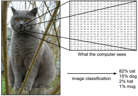
In computer vision, an image is represented by a number matrix, or a set of matrices, with each number in the matrix corresponds to the color value or intensity value of a pixel in the image.^[2] With this representation, linear algebra can be exploited for many CV operations from the most basic like transformation to very complex like feature extraction and motion tracking.

Additionally, with deep learning, a lot of new applications of computer vision have been introduced, including facial recognition, and object detection that is widely used in self-driving cars.^[3]

Applications of Computer Vision

Many systems and applications rely on computer vision, as they work extensively with image and video input for:

Navigation, e.g. autonomous cars to keep track of the road, detect pedestrians, and avoid collision with other vehicles.^[3]
Facial Detection, e.g. smartphones' camera software to focus on faces.^[4]
Visual Surveillance, e.g. detecting movements in security footage.^[4]
Automatic Inspection, e.g. measuring structures, modelling environment.^[4]
Searching, e.g. image search engines.^[5]

Typical Computer Vision Tasks

For a typical computer vision system, the tasks it aims to perform may include, but are not limited to, the following:^[6]

Geometric Image Transformation
Image Filtering
Image Classification
Structural Analysis and Shape Descripting
Feature Detection
Object Detection
Object Localization
Object Tracking

Core Problems in Computer Vision

Most problems requiring computer vision can be boiled down to one or a combination of the following core problems: image transformation, classification, localization, detection, and tracking.^[6]

This section introduces some of those core problems, and cites working examples for demonstration purposes. The examples use Open Source Computer Vision library (OpenCV) - containing implemented algorithm packages and utility functions for building computer vision applications. It is freely distributed and licensed for both academic and commercial use. The code examples cited in this section are written in Python, but OpenCV has API supports for C++ and Java as well.

Image Transformations

In many applications, image transformation is often the first step that standardizes the input and allows the application to subsequently perform more complex analysis.

Affine Transformation

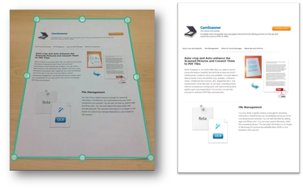
The most common transformations are scaling - resizing of image, translation - shifting of selected zones in image, rotation of image for an angle, and affine transformation - a combination of scaling, rotating, and translation, that reserves parallel lines in the original image.^[7]

Example: Perspective Warping using OpenCV

This example is extracted from "Building a Pokedex in Python: OpenCV and Perspective Warping" tutorial originally published on PyImageSearch on May 5, 2014. Refer to original tutorial here. All pictures and code snippets in this example belong to its original author, Adrian Rosebrock.

Suppose we have the picture of the Gameboy on the left, and we want to crop out just the game screen like the right side of the picture above. Notice that on the left the screen is slightly skewed, and we want to project it upright.

First of all, we need to have the coordinates of the 4 corners of the screen. This can be entered by hand, as OpenCV has helper functions for capturing mouse input; for example, user can use the mouse to click on the 4 corners of the game screen one by one and the application captures the coordinates of the clicked points. See more here. Then, we map the skewed image to a another rectangle frame pixel by pixel.

# We use numpy - a library for scientific computing with Python.
# OpenCV is referred to as 'cv2'.

# Declare a rectangle with the 4 corners - top-left, top-right,
# bottom-right, bottom-left, to represent the portion of the
# screen in the original image.
(tl, tr, br, bl) = rect

# Arbitrarily choose dimensions for the output image.
width = 100
height = 100

# Construct an array to store the desired coordinates of the 4
# corners of the screen after being transformed.
dst = numpy.array([
	[0, 0],
	[width - 1, 0],
	[width - 1, height - 1],
	[0, height - 1]], dtype = "float32")

# Calculate the perspective transform matrix and warp the
# portion of the original image to grab the up-right screen.
M = cv2.getPerspectiveTransform(rect, dst)
warp = cv2.warpPerspective(orig, M, (width, height))
# 'orig' here refers to the original image.
# 'warp' now stores the screen projected straight and up-right
# as seen in the picture above.

Image Classification

Image classification refers to the task of identifying the object present in an image. Typically, a predetermined set of possible objects is given and the classification of the image is the object that is most likely to exist in it.^[6]

source

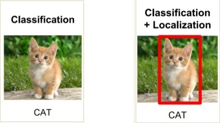
Image classification is often paired with object localization, which is the task of finding where in the image the object is. Many more complex problems in computer vision, such as object detection and segmentation, can be reduced to image classification and localization.^[6]

Fei-Fei Li, Andrej Karpathy & Justin Johnson (2016) cs231n, Lecture 8 - Slide 8, Spatial Localization and Detection (01/02/2016)

At the moment, there already exist classification/localization models that surpass trained humans. For example, in the 2014 ImageNet Large Scale Visual Recognition Challenge (ILSVRC),

Our results indicate that a trained human annotator is capable of outperforming the best model (GoogLeNet) with approximately 1.7% chance (p = 0.022).^[8]

Example: Classifying images using deep learning and OpenCV

This example is extracted from "Deep Learning with OpenCV" tutorial originally published on PyImageSearch on August 21, 2017. Refer to original tutorial here. All pictures and code snippets in this example belong to its original author, Adrian Rosebrock.

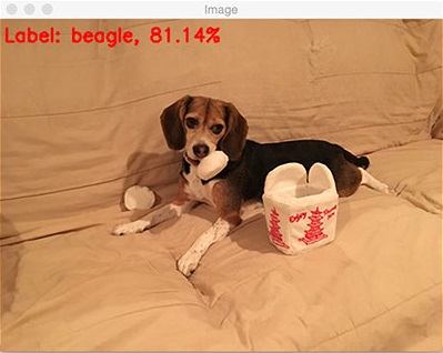
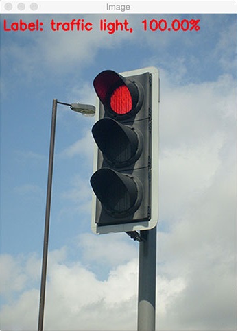
In this example, we use OpenCV and a pre-trained image classification model called the GoogLeNet.^[15] The goal of this example is to use the model to classify the object present in a given image. First, we load the image in question and the model, then we feed the image to the model and take the most confident prediction.

# Load the class labels from disk. Class labels is the actual
# name of a class of objects written in English, e.g. dogs,
# cats, helicopters. After taking the output from the model,
# we match that output with a label.
rows = open('./labels.txt').read().strip().split("\n")

# Load the model files from disk.
net = cv2.dnn.readNetFromCaffe('./googlenet.prototxt', './googlenet.caffemodel')

# Load the image and resize it to 224x224 to fit into the model.
image = cv2.imread('./image.jpg')
blob = cv2.dnn.blobFromImage(image, 1, (224, 224))

# Feed the image to the model.
net.setInput(blob)
preds = net.forward()
# 'preds' now stores the classes and their respective confident
# levels. We use numpy to grab the class with highest
# probability and store the index of that class in 'idx'.
idx = numpy.argmax(preds[0])[::-1]

# We get the name, or label, of the class, along with the
# probability, and put them on the image.
text = "Label: {}, {:.2f}%".format(classes[idx], preds[0][idx] * 100)
cv2.putText(image, text, (5, 25),  cv2.FONT_HERSHEY_SIMPLEX,
			0.7, (0, 0, 255), 2)

Some results:

Object Detection

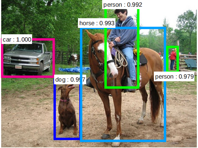
Object detection, as the name suggests, detects objects within an image. It combines image classification and localization in a sense that it gives the classification and bounding box (localization) of object in an image, but it does this to all instance of every known type of objects found in the image, instead of assuming only one type is present.^[9]

source

Obviously, object detection requires tremendous computing power compared to classification/localization; a naïve approach is to repeatedly classify and localize for every pixel in the image. In recent years, breakthroughs have been made towards a quicker and more efficient detecting algorithms, such as sharing computation on a whole image as can be seen in YOLO, SSD, and R-FCN. Notably, in 2016, the YOLO system named 'YOLO9000' was able to achieve real-time detection on motion pictures, and even able to detect object categories that it had never been trained for.^[9]

Example: Cat detection with OpenCV

This example is extracted from "Detecting cats in images with OpenCV" tutorial originally published on PyImageSearch on August 21, 2017. Refer to original tutorial here. All pictures and code snippets in this example belong to its original author, Adrian Rosebrock.

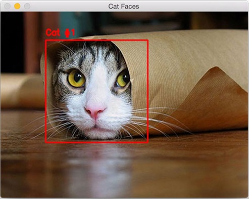
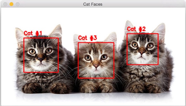
In this example, we apply object detection to find cats lurking in a given image using a Haar feature-based cascade classifier for face of cats. Haar cascade is a fast, efficient, and somewhat restricting, object detection method proposed by Paul Viola and Michael Jones.^[16] The classifier used below is pre-trained and shared by OpenCV; there are other classifiers for detecting various objects stored in OpenCV repository. In this example, for simplicity, we limit to detecting only 1 class of object, cats. In practice, one can combine many classifiers to detect multiple classes.

Since Haar cascade method relies on geometrical features of pixels, we convert the image to grayscale before processing it since color information is not relevant.

# Load the input image and convert it to grayscale.
image = cv2.imread('./image.jpg')
gray_image = cv2.cvtColor(image, cv2.COLOR_BGR2GRAY)

# Load from disk the Haar cascade detector for cat faces, then
# detect cats in the input image.
detector = cv2.CascadeClassifier('./haarcascade_frontalcatface.xml')
rects = detector.detectMultiScale(gray, scaleFactor=1.3,
	minNeighbors=10, minSize=(75, 75))
# 'rects' now contains all the rectangles that each corresponds
# to a cat's face detected in the image.

# For each rectangle in 'rects', we draw it into the original
# image and label the cat's number.
for (i, (x, y, w, h)) in enumerate(rects):
	cv2.rectangle(image, (x, y), (x + w, y + h), (0, 0, 255), 2)
	cv2.putText(image, "Cat #{}".format(i + 1), (x, y - 10),
		cv2.FONT_HERSHEY_SIMPLEX, 0.55, (0, 0, 255), 2)

Some results:

Object Tracking

Object tracking is the process of following and establishing the movement of a specific object of interest in a sequential set of images - typically a video clip or a real-time camera feed.^[10] It is crucial for autonomous driving systems such as self-driving cars or unmanned aerial vehicles (UAVs).

Tracking movement of cars with OpenCV

Object tracking algorithms can be divided into 2 categories: those applied to still backgrounds, and those to moving image frames such as those from a car camera.^[6] Algorithms in the former category typically compare subsequent images, extract the difference and deduce the movements, if any. Notable in this category are Optical Flow and the Waterfall algorithms.^[6] Moving image sources on the other hand require the tracking system to learn the relationships between each object's motion and the surroundings.^[4] In any case, all tracking systems require an initial detection of the object to track.^[6]

Example: Background subtraction for tracking with OpenCV

This example is extracted from "Background Subtraction " tutorial originally published on OpenCV's website. Refer to original tutorial here. All pictures and code snippets in this example belong to OpenCV organization.

In this example, different background subtraction methods are applied on a video track, differentiating the moving pedestrians from still background. The methods are 2 Gaussian mixture-based background/foreground segmentation algorithms developed by P. KadewTraKuPong and R. Bowden^[17] and Z.Zivkovic^[18]^[19], and a per-pixel Bayesian segmentation algorithm by Andrew B. Godbehere, Akihiro Matsukawa, and Ken Goldberg^[20].

The process is simple, the video is captured frame by frame and for each image frame, a subtraction mask is applied.

cap = cv2.VideoCapture('./test.avi')

# We use the algorithm by P. KadewTraKuPong and R. Bowden.
fgbg = cv2.createBackgroundSubtractorMOG()

# Use the below instead for Z.Zivkovic's algorithm.
# fgbg = cv2.createBackgroundSubtractorMOG2()
# Use the below instead for the algorithm by Godbehere et al.
# fgbg = cv2.createBackgroundSubtractorGMG()

while(1):
    ret, frame = cap.read()

    if ret:
      fgmask = fgbg.apply(frame)
      cv2.imshow('frame',fgmask)
      k = cv2.waitKey(30) & 0xff
      if k == 27:
          break
    else:
      break

Some results:

Original frame:

With BackgroundSubtractorMOG:

With BackgroundSubtractorMOG2:

With BackgroundSubtractorGMG:

GPU-Accelerated Computer Vision

For computer vision systems, digital images are often translated into matrices, whose nature depends on the chosen color presentation. For example, an image in the RGB (Red, Green, Blue) color space will be presented by 3 matrices, each contains the color intensity of the individual pixels with regards to red, green, or blue. There are other color representations, such as the CMYK or the HSV that annotates the pixels' Hue, Saturation, and Value.^[1]

Underneath, all computer vision algorithms deal with images as matrices, thus employ theories in Linear Algebra to process images. In computer hardware, there is a class of computing units that specializes in matrix operations called the Graphics Processing Units (GPUs) - their main purpose is to speed up heavy graphical tasks such as video rendering, gaming, or 3D modelling. Therefore, GPUs are well-suited to serve as computer vision computing units.^[11]

Most prominent computer vision libraries such as OpenCV, dlib, or VisionWorks support the use of GPUs in the computing process. For example, OpenCV has APIs that allow a kernel process running on the CPU to transfer image matrices to one or more GPUs to perform heavy functions such as Gaussian filtering or image stitching.^[12] Hardware manufacturers have even tried to ease the image transferring process between CPU and GPU, by introducing system memory regions accessible to both CPU and GPU.^[13]

What's Next?

There is an abundance of resources to learn and apply computer vision; however, not all of them are free or beginner-friendly. This section mentions some great courses and tutorials that are freely accessible at the time of writing. If you are a starter, it is recommended that you follow these steps for your learning journey:

Firstly, you should acquire basic familiarity in Python, C++, or Java, as most tutorials and courses in CV use one of those languages:

Next, it is necessary that you gain some basic understandings in Linear Algebra:

Linear Algebra by Khan Academy

After getting comfortable with the language and the math, you should start with an entry-level computer vision course. This Udacity class pairs theoretical parts with very practical hands-on exercises: